Machine Learning Note
Machine Leaning
Overview
What’s Machine Learning
“Filed of study that gives computers the ability to learn without being explicitly programmed.” —— Arthur Samuel (1959)
ML is subset of AI that uses algorithms and requires feature engineering
Categories
- Supervised Learning
- Semi-Supervised Learning
- Unsupervised Learning
- Reinforcement Learning
Techniques
- Classification
- Regression
- Clustering
- Association
- Anomaly detection
- Sequence mining
- Dimension reduction
- Recommendation systems
Data
Data is a collection of raw facts, figures, or information used to draw insights, inform decisions, and fuel advanced technologies.
Data is central to every machine learning algorithm and the source of all the information the algorithm uses to discover patterns and make predictions.
Process Lifecycle of ML Model
- Problem Definition
- Data Collection
Data Preparation
- Clean data to remove irrelevant data
- Remove extreme values
- Missing values should be removed or replaced
- Each data column should be in the proper format
- Create new features
- Exploratory Data Analysis (EDA, all about graphing data and doing statistical inference. e.g. Correlation Analysis)
- Identify how to split up the data into training and test sets
Model Development
- Explore existing frameworks
Model Evaluation
- Evaluate model on never-before-seen data
- Test set
- Small scale test in reality
- Evaluate model on never-before-seen data
Model Deployment
- Continue to track model performance
- Retrain model based on new infomation
In reality, the model lifecycle is iterative, which means that we tend to go back and forth between these processes.
####
ML Tools
ML tools provide functionalities for ML pipelines, which include modules for:
- Data processing and building
- Evaluating
- Optimizing
- Implementing ML models
ML programming language is used to build ML models and decode data patterns
Machine learning ecosystem
- Create and tune ML models
- NumPy: Numerical computations on data arrays
- Pandas: Data analysis, visualization, cleaning, and preparation
- SciPy: Computing for optimization, integration,and linear regression
- Scikit-learn: Suite of classification, regression,clustering, and dimensionality reduction
Deep learning
- Designing, training, and testing neural network-based models
- TensorFlow: Numerical computing and large scale ML
- Keras: Implementing neural networks
- Theano: Defining, optimizing, and evaluating mathematical expressions involving arrays
- PyTorch: Computer vision, NLP, and experimentation
Computer Vision
Computer Vision tools are used for tasks such as:
- Object detection
- Image classification
- Facial recognition
- Image segmentation
All of the deep learning tools can be tailored to computer vision applications.
- OpenCV: Real-time computervision applications
- Scikit-image: Image processing algorithms
- TorchVision: Popular data sets, image loading, pre-trained deeplearning architectures, and image transformations
Natural language processing
NLP tools help developers and data scientists build applications that understand, interpret, and generate human language.
Tools:
- NLTK: Text processing,tokenization, and stemming
- TextBlob: Part-of-speechtagging, noun phrase extraction,sentiment analysis, andtranslation
- Stanza: Pre-trained models for tasks such as part-of-speech tagging, named entity recognition, and dependency parsing
Generative AI
Leverage AI to generate new content based on input data. For example:
- Hugging face transformer: Text generation, languagetranslation, and sentiment analysis
- ChatGPT: Text generation, building chatbots, etc
- DALL-E: Generating images from text descriptions
- PyTorch: Uses deep learning to create generative models such as GANs (Generative Adversarial Networks) and transformers
Data Preprocess | TMPTitle
Feature Scaling
特征缩放 (Feature Scaling) 是机器学习中数据预处理的一个重要步骤,目的是将数据集中各个数值型特征(独立变量)的取值范围(量纲和数量级)统一或规范化到一个相似的区间内,避免某些特征因为其数值范围较大而在模型训练中占据主导地位,从而提高模型的训练效率和性能。
Key Purposes
- 防止特征支配 (Prevent Feature Dominance): 如果特征的取值范围相差很大(例如,年龄在 0-100 之间,而收入在数万到数百万之间),数值较大的特征会在基于距离的算法(如 k-近邻 (k-NN) [1]、支持向量机 (SVM) 、K-均值聚类 )中对距离计算产生不成比例的影响,掩盖其他特征的重要性。
- 加速优化算法收敛 (Speed Up Convergence): 对于使用梯度下降 (Gradient Descent) 的算法(如线性回归、逻辑回归、神经网络 ),特征缩放可以使损失函数的等高线图更接近圆形,而不是细长的椭圆形,从而使梯度下降能够更快地找到最优解(即更快地收敛)。
- 改善模型性能 (Enhance Model Performance): 特征缩放有助于提高模型的准确性和稳定性。
Common Methods
- Mean Normalization(均值归一化)
where $\mu$ is the mean of the feature $X$
which makes $X_{new} \in [-1, 1]$, $\mu_{new} = 0$
e.g. $300 \leq x \leq 200$, which $\mu = 600$, thus $\frac{300 - 600}{2000 - 300} = -0.18 \leq x_{new} \leq 0.82 = \frac{2000 - 600}{2000 - 300}$
- Z-Score Normalization/Standardization(Z-分数标准化/标准化)
where:
$\mu$ is the mean of the feature $X$
$\sigma$ is the standard deviation of the feature $X$, where$\sigma = \sqrt{\frac{\sum_{i=1}^{N}(X_i-\mu)}{N}}$
which makes $\mu_{new} = 0$, $\sigma_{new} = 1$, $X_{new} \in (-\inf, \inf)$ (but mostly $X_{new} \in [-3, 3] or [-4, 4]$)
Model Training | TMPTitle
Regularization
正则化(Regularization)是机器学习中用于解决过拟合 (Overfitting) 问题、提高模型泛化能力 (Generalization) 的一类技术。
Main Principle
正则化的最常见实现方式是,在模型训练时,给原有的成本函数 (Cost Function) 额外增加一个惩罚项(或正则化项)
\[totalCost = originalCost + \lambda \times regularizationTerm\]where $\lambda$ is the regularization parameter
Regularization Type
L1 正则化(L1 Regularization / LASSO Regression)
- 惩罚项是模型所有权重系数的绝对值之和。
- 它有一个重要的特性:能够将一些不重要特征的权重直接降为零,从而实现特征选择 (Feature Selection),让模型更加稀疏和易于解释。
L2 正则化 (L2 Regularization / Ridge Regression)
- 惩罚项是模型所有权重系数的平方和。
- 它倾向于使模型的权重趋近于零但不会变为零,从而使所有特征对结果都有一定的贡献,但不会有过大的权重,达到权重均衡分配的效果。
- e.g. n: the count of features m: the count of items Function: $f_{\vec{w}, b}(\vec{x}) = \vec{w} \cdot \vec{x} + b$ Cost Function: $J(\vec{w}, b)=\frac{1}{2m}\sum_{i=1}^{m}(f_{\vec{w}, b}(\vec{x}^{(i)})-y^{(i)})^2 + \frac{\lambda}{2m}\sum_{i=1}^{n}w_j^2$
Evaluating and Choosing Models
Dataset usually will be split into three parts: Training Set, Cross Validation Set(Validation Set\Development Set\Dev Set), Test Set.
From now on, I will use linear regression as an example to develop.
n: the count of features
m: the count of items
Function: $f_{\vec{w}, b}(\vec{x}) = \vec{w} \cdot \vec{x} + b$
Training Error: $J_{train}(\vec{w}, b)=\frac{1}{2m_{train}}\sum_{i=1}^{m_{train}}(f_{\vec{w}, b}(\vec{x}{train}^{(i)})-y{train}^{(i)})^2$
Cross validation Error: $J_{cv}(\vec{w}, b)=\frac{1}{2m_{cv}}\sum_{i=1}^{m_{cv}}(f_{\vec{w}, b}(\vec{x}{cv}^{(i)})-y{cv}^{(i)})^2$
Test Error: $J_{test}(\vec{w}, b)=\frac{1}{2m_{test}}\sum_{i=1}^{m_{test}}(f_{\vec{w}, b}(\vec{x}{test}^{(i)})-y{test}^{(i)})^2$
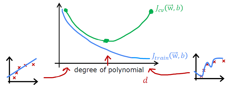
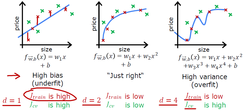
Model Selection
- Degree of polynomial $d$
The $d$which has the lowest $J_{cv}(w^{
The estimated generalization error using the test set will be optimistic, because of the way to estimate how well this model performs is to report the test set error $J_{test}(w^{<?>}, b^{<?>})$, which means an extra parameter d (degree of polynomial) was chosen using the test set. That’s the reason why we need split data set into three parts instead of two parts.
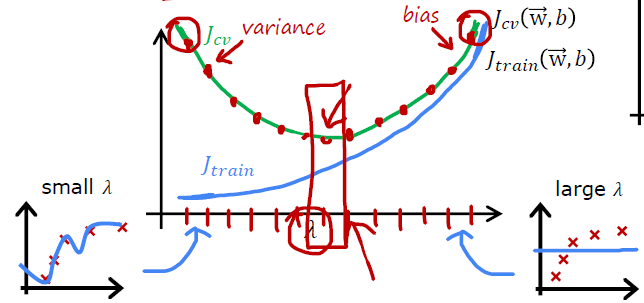
- Regularization parameter $\lambda$
The $\lambda$which has the lowest $J_{cv}(w^{<\lambda>}, b^{<\lambda>})$is the best regularization parameter.
Bias and Variance
Baseline
baseline 指的是一个最简单、最基础、最容易实现的模型或方法,用于作为后续更复杂模型的比较标准。
例如做二分类,训练集中有 70% 都是「负类」,那么 baseline 可以是:永远预测「负类」,准确率立刻有 70%。如果你训练的深度神经网络只有 65%,那就说明模型出现问题了。
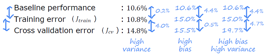
Bias
Bias (偏差) 是模型的系统性误差,衡量了模型的预测与真实值的平均偏离程度,其数学定义为:
\[Bias(x) = \mathbb{E}[\hat{f}(x)] - f(x)\]期望 $\mathbb{E}[\hat{f}(x)]$ 指的是:在“不同训练集”上训练同一个模型后,对同一个输入 xxx 得到的“预测值的平均值”
High Bias: 模型太简单,无法很好地拟合数据
- 欠拟合 (Underfitting)
- $J_{train}$is high
- $J_{cv}$is high
Low Bias: 模型足够复杂,能更好地逼近真实模式
Variance
Variance (方差) 是模型对数据集扰动的敏感程度,衡量了模型在不同训练集之间的预测波动情况,其数学定义为
\[Var(x) = \mathbb{E}[(\hat{f}(x)-\mathbb{E}[\hat{f}(x)])^2]\]High Variance: 模型对训练数据太敏感
- 过拟合 (overfitting)
- $J_{train}$is low
- $J_{cv}$is high
Low Variance: 模型较稳定,不会因为数据变化而乱变
Learning Curves
学习曲线(Learning Curve)是一种非常重要的诊断工具,用于评估模型在不同规模训练集上的性能表现。
经典的学习曲线是:
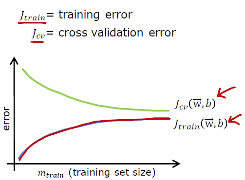
可以看出:
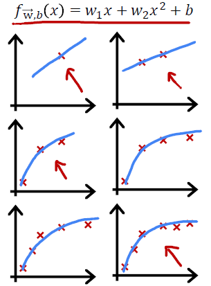
- 随着$m_{train}$变大,$J_{train}(\vec{w},b)$变大:在特定的模型下,如右图,$m_{train}$越大该模型越无法拟合所有训练集数据
- 随着$m_{train}$变大,$J_{cv}(\vec{w},b)$变小:在特定的模型下,如右图,$m_{train}$越大该模型越容易 generalization,越容易预测到训练集之外的数据(Cross Validation Set)
- $J_{cv}(\vec{w},b) > J_{train}(\vec{w},b)$:模型参数拟合到训练集,自然训练集误差应小些
High bias
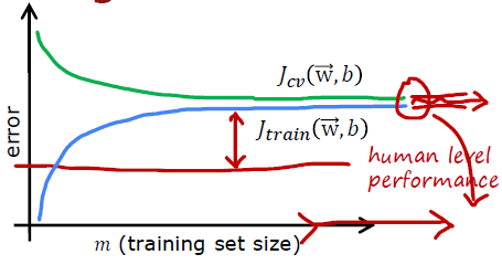
If a learning algorithm suffers from high bias, getting more traning data will not (by itself) help much.
High variance
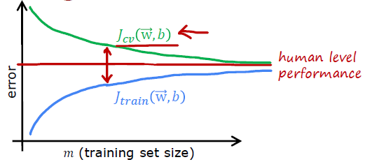
if a learning algorithm suffers from high variance, getting more training data is likely to help.
Debugging a learning algorithm
Transfer Learning
迁移学习是一种机器学习技术,通过在一个任务或数据集上获得的知识来提升模型在另一个相关任务或不同数据集上的性能。换句话说,迁移学习利用在一个场景中学到的知识来提升另一个场景中的泛化能力 (e.g. 用来辨识汽车的知识(或者是模型)也可以被用来提升识别卡车的能力)。
- Download neural network parameters pretrained on a large dataset with same input type (e.g., images, audio, text) as your application (or train your own).
- Further train (fine tune) the network on your own data.
Skewed Datasets
偏斜数据集(Skewed Datasets)是指该数据集中某一个类别的样本数量远远多于另一个类别。(e.g. Rare disease, of the 1,000 patient samples, only 5 were diseased [positive samples] and 995 were healthy [negative samples].)
偏斜数据集会导致准确率(Accuracy)失效,从而产生误导。
如果一个数据集有 99% 的样本是“非癌症”,只有 1% 是“癌症”。
- 如果我写一个愚蠢的算法,永远只预测 “非癌症”(即忽略所有输入特征)。
- 该算法的准确率依然高达 99%。
- 但是,这个模型完全没有用,因为它一个癌症病人都没找出来。
这就是准确率悖论。在偏斜数据集中,模型倾向于只预测“多数类”来获得高分,而忽略了我们真正关心的“少数类”。
How to Evaluate
- 混淆矩阵 (Confusion Matrix)
- 精确率 (Precision): 在预测为正的样本中,有多少是真的正样本?(预测准不准)
- 召回率 (Recall): 在所有真的正样本中,你找出了多少?(找的全不全)
- F1 分数 (F1-Score): 精确率和召回率的调和平均数
Trade-off Precision and Recall
Logistic regression: $0 < f_{\vec{w}, b}(\vec{x}) < 1$
Predict 1 if $f_{\vec{w}, b}(\vec{x}) \geq threshold$
Predict 0 if $f_{\vec{w}, b}(\vec{x}) < threshold$
Usually the threshold will be set 0.5
Suppose we want to predict 𝑦 = 1 (rare disease) only if very confident. a.k.a. Increase the threshold => Lower FalsePos, Higher FalseNeg => Higher Precision, Lower Recall
Suppose we want to avoid missing too many cases of rare disease (when in doubt predict 𝑦 = 1) a.k.a Decrease the threshold => Higher FalsePos, Lower FalseNeg => Lower Precision, Higher Recall
So, by choosing the threshold, we can make different tradeoffs between precision and recall
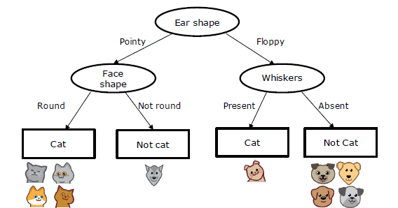
Decision Trees
决策树是一个预测模型;它代表的是对象属性与对象值之间的一种映射关系。树中每个节点表示某个对象,而每个分叉路径则代表某个可能的属性值,而每个叶节点则对应从根节点到该叶节点所经历的路径所表示的对象的值。 e.g.
Decision 1: How to choose what feature to split on at each node?
- Maximize purity (or minimize impurity)
Decision 2: When do you stop splitting?
- When a node is 100% one class
- When splitting a node will result in the tree exceeding a maximum depth
- When improvements in purity score are below a threshold
- When number of examples in a node is below a threshold
Entropy as a measure of impurity
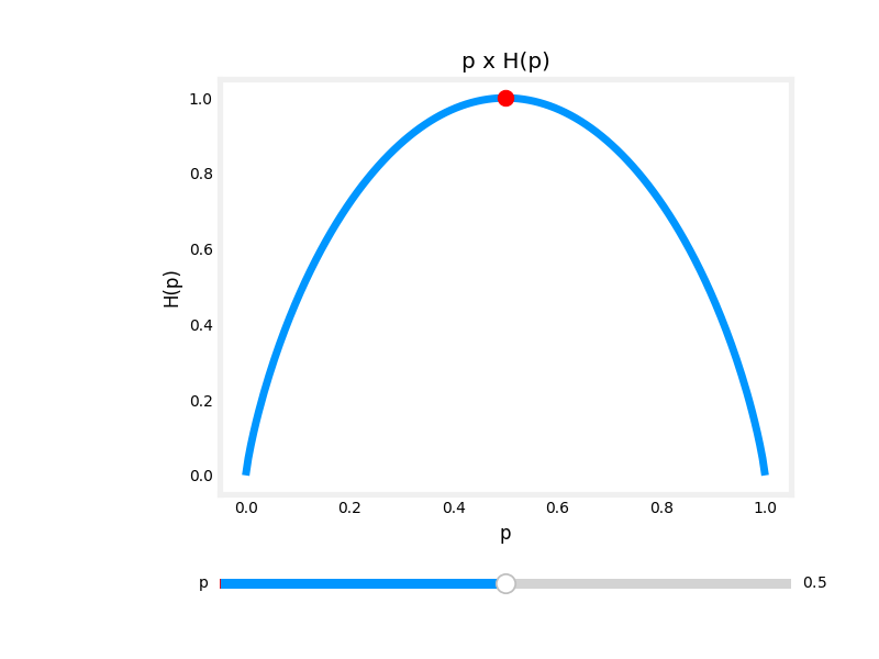
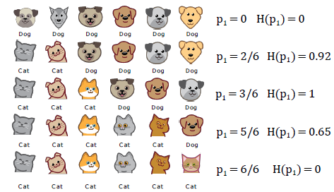
$p_1$ = fraction of examples that are cats $p_0 = 1 - p_1$
\[H(p_1)=-p_1\log_2(p_1)-p_0\log_2(p_0)=-p_1\log_2(p_1)-(1-p_1)\log_2(1-p_1)\]Note: $’‘0\log(0)’‘=0$
1
2
3
4
5
def entropy(p):
    if p == 0 or p == 1:
        return 0
    else:
        return -p * np.log2(p) - (1- p)*np.log2(1 - p)
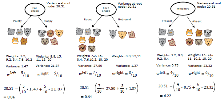
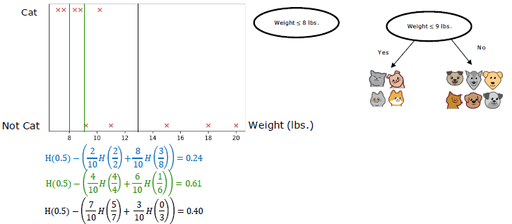
Information Gain
信息增益是指一个变量的单变量概率分布相对于给定另一个变量的条件分布的 Kullback-Leibler 散度的条件期望值。公式如下:
\[Info\;Gain=H(p_1^{root})-(w^{left}H(p_1^{left})+w^{right}H(p_1^{right}))\]e.g.
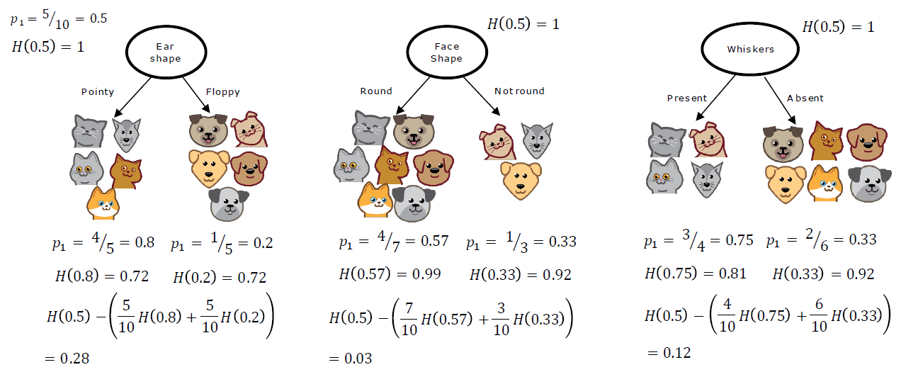
What INFORMATION GAIN measures is the reduction in entropy that you get in your tree, resulting from making a split
Step of building decision tree
- Start with all examples at the root node
- Calculate information gain for all possible features, and pick the one with the highest information gain
- Split dataset according to selected feature, and create left and right branches of the tree
Keep repeating splitting process until stopping criteria is met:
- When a node is 100% one class
- When splitting a node will result in the tree exceeding a maximum depth
- Information gain from additional splits is less than threshold
- When number of examples in a node is below a threshold
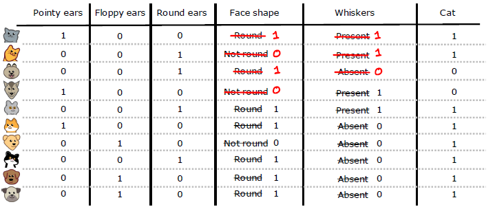
One-Hot Encoding of categorical features
One Hot Encoding: If a categorical feature can take on 𝑘 values, create 𝑘 binary features (0 or 1 value).

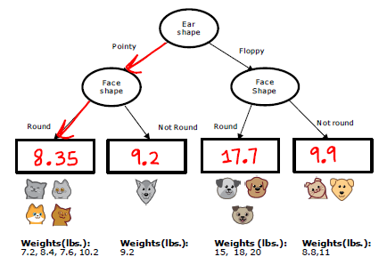
Continuous features
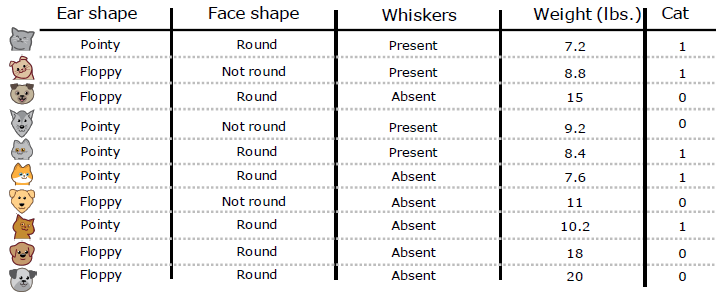
Regression with Decision Trees: Predicting a number